On October 7 the BPER FORUM Monzani in Modena hosted the Particleworks Experience. Six talks with recordings asked three questions: where does the heat go, where does the air go, and where does the material wear?
The speakers came from a bearing maker, a pump manufacturer, a hydropower research project and several engineering firms. Each put the simulation next to a thermocouple, an optical sensor or a worn prototype, and stated the gap. Every “Watch this moment” link plays the recording at that second in a floating player. The full slides are on the proceedings page.
Closing the thermal model
Two talks closed a thermal model with the same trick: oil and metal never run on the same clock. The oil is simulated briefly, its heat-transfer map goes into a steady solution of the solids, and the result is compared with measurements. The SKF talk, in between, tests the heat-transfer coefficient such models rely on.

CHT Analysis of a Reciprocating Pump
An industrial pump bathed in oil, no thermal data on its contacts, and a model that counts as finished only when the oil neither gains nor loses heat.
Volumetric pumps for food, chemical and waste-water plants run all day at a fixed operating point. What goes wrong first is thermal: seals degrade, components overheat. Inside the pump the oil is the only link between hot and cold parts, and every watt finally leaves through natural convection. R&D CFD, with its customer Comet, wanted a thermal model of the real operating point and a method it can reuse on the next pump.
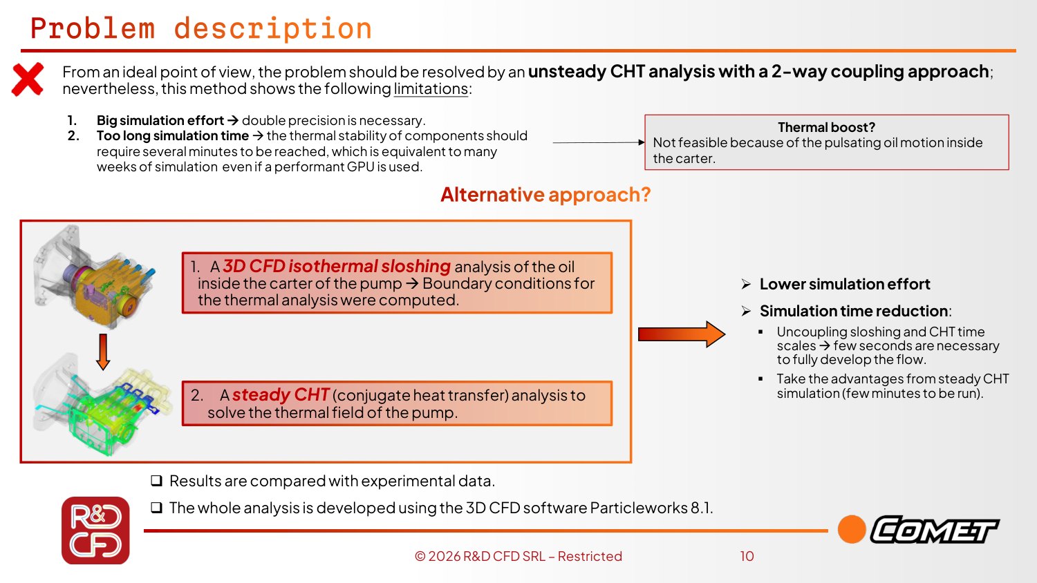
A fully coupled unsteady run was ruled out: it needs double precision, and sloshing lives in seconds while heat lives in hours, so the run would be far too long. The problem was cut in two. A few seconds of Particleworks sloshing give the heat-transfer map; a steady conjugate-heat-transfer (CHT) solution then converges in minutes.
Do not guess where the heat is born
Loads on the contacts were not available. Trial and error was rejected as stochastic and unvalidated; a dynamic analysis of the pump with friction coefficients from the literature gave a power split instead, with far fewer free variables. The largest share sits on the piston–block pair, the contact that is also critical in the test.
Two independent checks, not one
First the thermocouples, compared one to one at the test positions. Then the oil: it is a heat carrier, not a heat sink, so the heat taken from the shaft must equal the heat given to the housing. If either fails, the power, the oil temperature or the ambient HTC is scaled and the loop restarts.
“The oil is not a heat sink. All the heat carried by the oil should be exchanged with the other components of the pump, so the balance of the oil should be equal to zero.”
Leonardo Lanciotti 21:19 Watch this moment
The model shows where the seals suffer
All thermocouples align; the worst, the open-side bearing, is off by about 5–6 °C and points to a local particle refinement as the next step. The shaft sits at 70–80 °C as in the test, and a hot spot at the piston–seal contact shows up where seals degrade abnormally in service.
Cheap enough to do by hand
Three to five iterations were enough, and a steady CHT takes minutes on a GPU. Once the model exists, a case takes about an hour and a half.
“Sometimes the setup is longer than the simulation itself. But, of course, we are talking about one hour and a half once the model is defined.”
Leonardo Lanciotti 20:20 Watch this moment
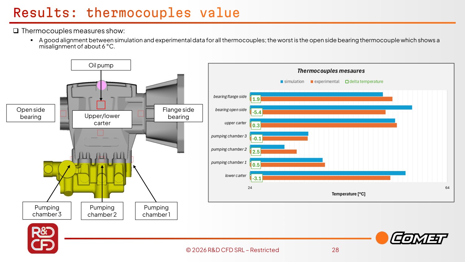
The oil balance is checked on a uniform surface mesh built from the HTC map. Heat enters the oil from the shaft and leaves it into the housing; the two flows must be equal, so the balance closes to 0 W.
In short
- Sloshing and heat are decoupled: seconds of oil, minutes of steady CHT.
- The oil balance at zero is the check that does not depend on the thermocouples.
- About 1.5 h per case once the model exists; automation with Python is the natural next step.

Integrating Particleworks into SKF Engineering Tools: Part I
Before trusting a heat-transfer coefficient inside a bearing tool, SKF tested it on the simplest cases that exist, and found that the answer depends on where you read it.
SKF frames the problem with one number: about 20 % of the world’s energy is lost to friction. Bearings fight friction, but even a good bearing is a source of heat, and temperature then shapes everything: the lubricant film, thermal expansion and the extra load it brings, and life, because every degree more shortens the life of the lubricant and of the bearing.
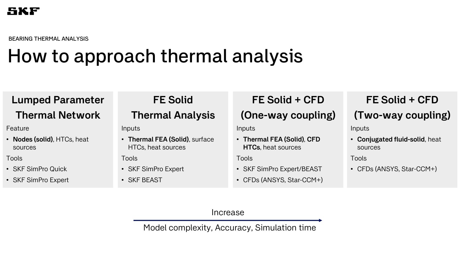
Thermal analysis is a ladder, from lumped networks that answer in real time, through finite elements with HTCs from analytical formulas, to CFD coupled one way and finally two ways, where answers take days or weeks. SKF’s next rung is one-way: its in-house bearing tool BEAST provides dynamics and heat sources, Particleworks provides the HTC maps. Part I of the study is the verification of those HTCs. Rolling bearings cannot be measured easily, so the references are classic cases: a sphere in a cross-flow, and two concentric cylinders.
One sphere, many answers
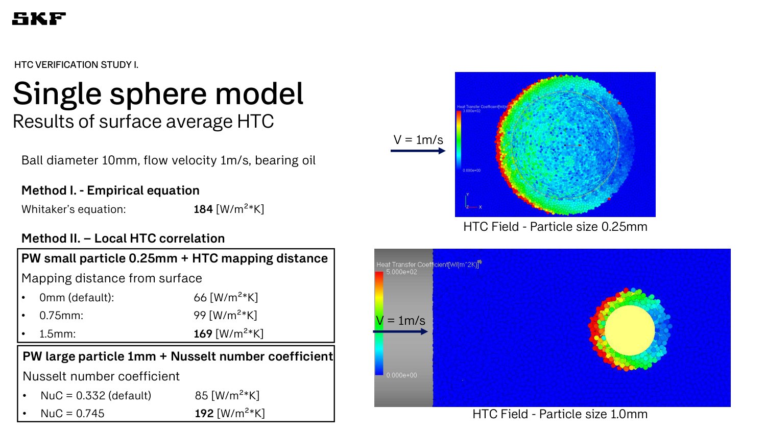
The reference is the Whitaker correlation: 184 W/m²K. Particleworks’ local-correlation method reads the velocity of particles next to the wall, which tends to zero there, so it reports a low HTC: 66 at the wall, 169 when sampled 1.5 mm away. With coarser particles the default is 85, and raising the Nusselt coefficient lifts it to 192.
“Imagine if you apply a non-slip condition very close to the wall: the velocity is approaching zero, so you get a very low Reynolds number and therefore a very low HTC. There’s nothing wrong with it. This is just the nature of the method.”
Lijun Cao 24:48 Watch this moment
The heat-flux method converges, at a price
Solving the temperature field and reading the heat flux does not care about mapping distance, and improves with refinement (75 → 127 W/m²K from 0.5 to 0.25 mm, against 180 for Ansys Fluent). But a thermal particle is heavier than a flow-only one, so further refinement was too expensive. Local refinement was disappointing, and is improved in the new release.
Concentric cylinders: defaults were enough
Heat transfer here is governed by the vortex pattern, and published correlations each hold only in a parameter range. The vortices appeared with mostly default settings (watch the Courant limiter). Across four radius-ratio and speed cases Particleworks sits between −7 % and +28 % of the correlation, a spread comparable with Fluent (−8 % to +17 %).
A lucky trial in the field
On a confidential customer case, a large oil system with spherical thrust bearings, SKF simply imported the power loss from its bearing software as a heat source and let Particleworks run. The temperature map was something the customer could relate to.
“We never tried; we just pushed the button and saw what happens with default settings. [...] It worked. [...] Maybe we’re just being lucky in that occasion.”
Fabrizio Mandrile 45:00 Watch this moment
In short
- Be conscious of what drives a discrepancy: mapping distance, Nusselt coefficient and refinement each moved the sphere HTC by a factor of two or more.
- Next: a segmented bearing, ideally with a cyclic boundary condition (requested), then a full bearing with multi-layer refinement.
- The correlation is a reference, not the truth.

Study of the Lubrication on Carrier Roller using a CFD 3D-MPS Method
A sealed, partly filled oil bath heats itself as it turns. TrackOne maps its temperatures in about a day per case, and a bench test shows where the model can be trusted.
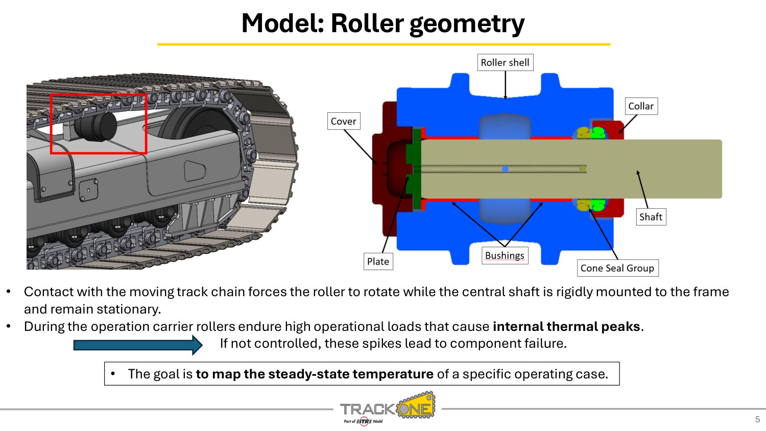
The carrier roller holds up the track chain of an excavator. The chain forces the shell to rotate around a fixed shaft; seals, bushings and a partial oil fill keep metal from touching metal. Under load, the friction creates internal thermal peaks, and “if not controlled, the spikes lead to component failure”. The goal was a steady-state temperature map for a given operating case.
Because the oil only partly fills the roller, it is thrown and fragmented against the walls as the shell turns. That, and the narrow passages in cover, bushing and shaft, is why TrackOne, with the Enzo Ferrari engineering department of Unimore, chose a meshless method.
Fluid and solid do not share a clock
The oil reaches its pattern in milliseconds, the metal in hours, so a straight unsteady CHT is prohibitive. The answer is an iterative steady CHT with two phases: the oil alone produces average HTC and near-wall temperature maps (a few hours), then the solids alone are solved with those maps (a few minutes). The loop stops when the solid field no longer changes, after three to four iterations.
“The temporal scale of the fluid was very different from the temporal scale of the solid. So we decided to use an iterative steady-state CHT.”
Leonardo Tiberi 9:53 Watch this moment
A moving contact, rewritten for a steady model
The chain touches only the top of the roller shell. A steady run with that contact alone would give “an unrealistic and unbalanced temperature map”. TrackOne spreads the cooling over the whole circumference and corrects it with a scale factor τ (footprint area over contact area) and an equivalent thermal contact resistance.
Case 1 within about 12 %, case 2 below 7 %
On the bench, with sensors outside and a probe in the oil, case 1 shows good convergence with a slight underestimation of the roller shell and the oil (errors up to about 12 %). Case 2, at higher speed and lower load, is excellent: all errors below 7 %. About one day per case.
“There is a good convergence between simulated and bench test temperature, with a slight underestimation of the roller shell and the internal oil temperature.”
Leonardo Tiberi 14:10 Watch this moment
What is not resolved
In the Q&A the numerics were questioned: the smallest gap, between shaft and bushing, is not resolved with particles. Next steps: oil rheology evolution, coupling with a FEM solver for deformation, and critical operating conditions.
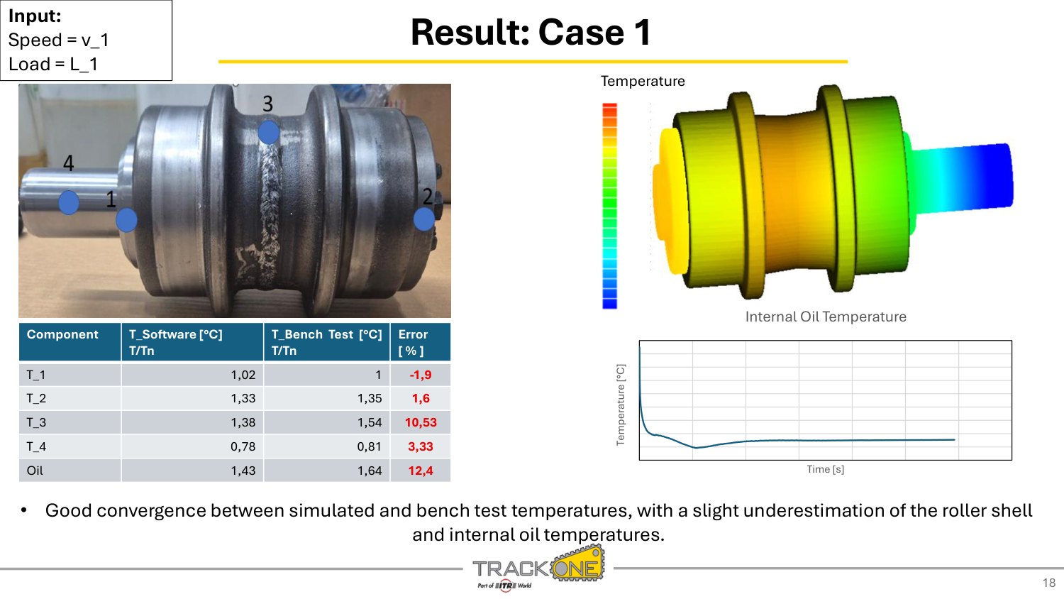
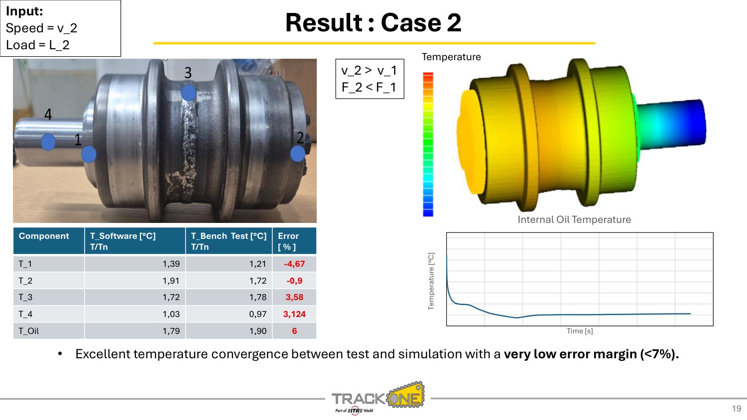
Two closures keep the steady model realistic. The chain loads only the top of the shell, so the cooling is spread over the whole circumference and corrected with a scale factor. Air convection on exposed components follows an analytical law in the component velocity v, and oil viscosity follows an Arrhenius–Vogel law in temperature.
In short
- Phase 1 (oil, hours) and phase 2 (solids, minutes) alternate until the solid field is stable.
- Errors are reported component by component: up to about 12 % in case 1, below 7 % in case 2.
- Next: rheology evolution, FEM coupling, critical conditions.
Measure it before you simulate it
Aeration changes viscosity, density, film thickness and oxidation rate. The afternoon showed how to get a measured number for it before asking the model to predict it.

Direct Optical Air-in-Oil Measurement as an Enabler for Accurate Simulation of Gearings and Hydraulic Systems
Two oils with the same air content can behave very differently. Calibrate the aeration model on bubbles, not on a percentage.
Air in oil is a multi-scale problem: root causes and effects sit in different places and develop over time. A gas phase changes the density and viscosity of the oil, so efficiency drops; it brings cavitation and NVH problems; it exposes the oil to thermal and chemical stress, with oxidation in the long run; and it makes the lubricant film unreliable where the gear needs it. Particleworks has an aeration module that predicts generation, transport, coalescence and disappearance of bubbles.
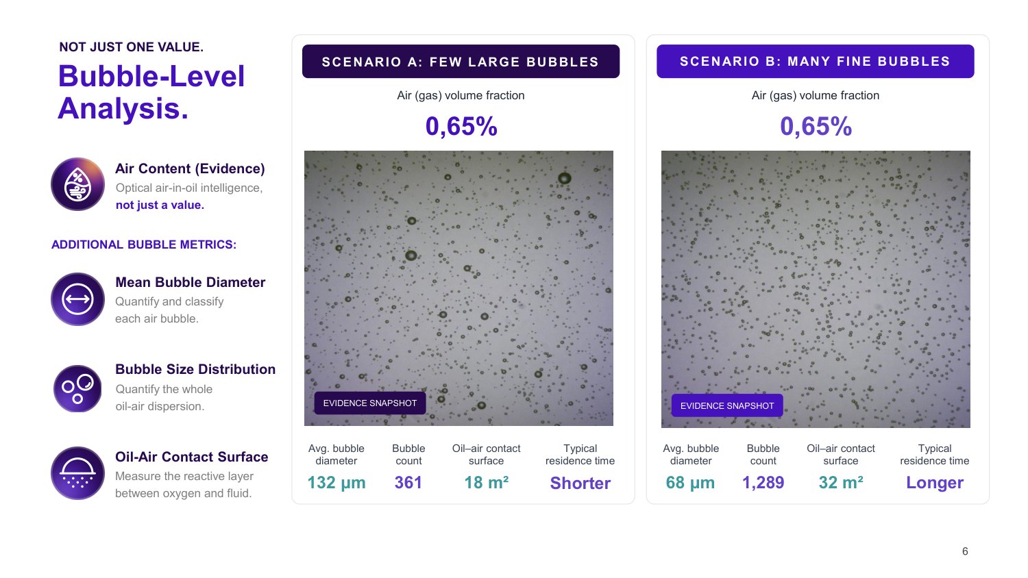
What was available until now was a single number, the air content. deepfluid’s optical sensors, in the laboratory, on the test bench and in the field, take snapshots of every bubble and give the bubble count, the size distribution, the mean diameter and the oil–air contact surface, with the snapshot as evidence.
One air content, two bubble populations
In scenario A, 361 bubbles of 132 µm offer 18 m² of oil–air surface. In scenario B, 1,289 bubbles of 68 µm offer 32 m² for the same volume of air. The surface is where oxidation happens, so oil aging, cavitation and compressibility differ although the percentage is identical.
“Those 0.65 percent of air content can look very different: pretty big bubbles with a wide deviation in sizes, or very, very small bubbles all the time. And this changes your system behavior pretty much.”
Dr. Lukas Hafner 5:25 Watch this moment
Measure, calibrate, then simulate
The aeration model has many coefficients, and two things are calibrated: the total amount of air generated and the bubble-size distribution. Simulation then gives the global picture (flow paths, recirculation, aeration hot spots) while the sensor measures what is happening at one point: “measured data does not replace the simulation”.
A differential gear, before and after
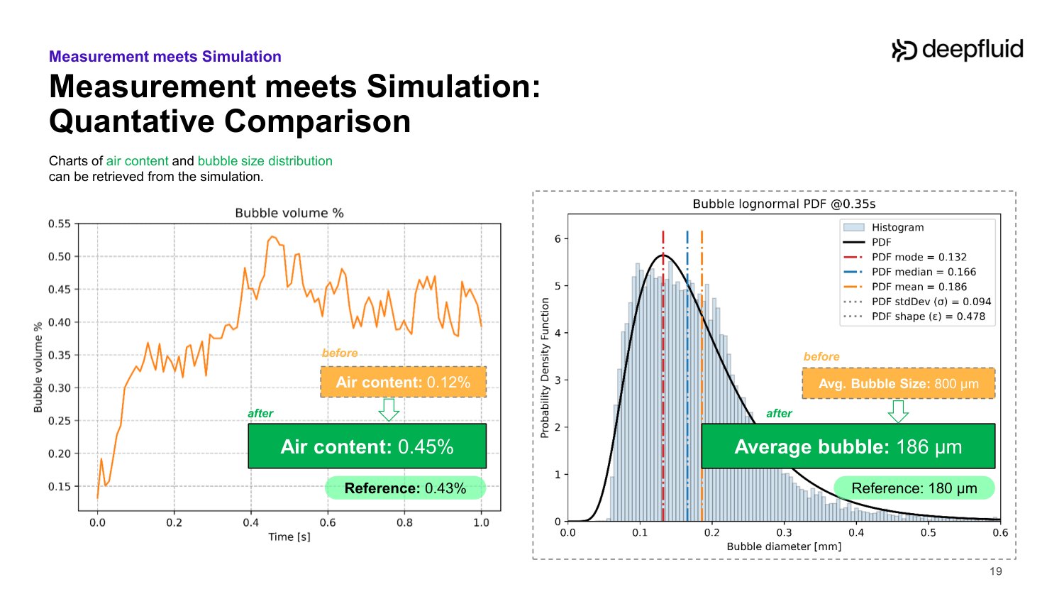
In a differential gear in a pool of oil, the default coefficients gave 0.12 % air with 800 µm bubbles. After calibration on the measurement: 0.45 % against 0.43 % measured, and 186 µm bubbles against 180 µm. The bubble motion and the recirculation under the gear are visibly better captured.
How far does a calibration travel?
Geometry: no problem. Speed: coefficients scale with the velocity ratio from a calibrated reference. Additive package: no, because Particleworks does not solve chemistry; a new additive or anti-foam means a new calibration. Temperature: an open point, and the trend can even change sign from oil to oil.
“For one and the same base oil with different additive packages, you can have an increase in air content with an increase in temperature. But with the other one, you get a decrease in air content with an increase in temperature.”
Dr. Lukas Hafner 24:22 Watch this moment
In short
- Calibrate two things: total air generated and bubble-size distribution.
- Scale with speed from a reference; recalibrate for a new additive package; temperature scaling is open.
- The sensor complements the simulation: a local measurement against a global view.
Where it wears, and what that costs
Two very different machines, one question: can a particle simulation say where the hardware wears and how much performance it loses?

Moving Particle Simulation of Eroded Pelton Runners
Europe’s hydropower is ageing and silting up. HES-SO uses Particleworks to put a number on what sediment erosion costs a Pelton runner in torque.
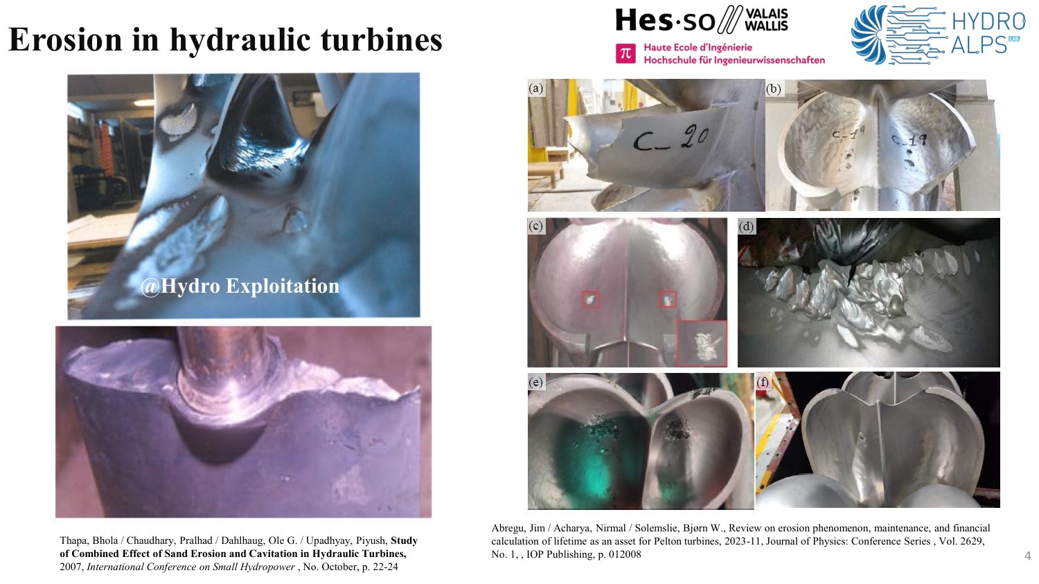
ReHydro is a Horizon Europe project of 18 partners, coordinated by SINTEF, to refurbish and modernise European hydropower. The fleet is about 50 to 55 years old and now has to balance solar and wind, and as glaciers retreat more sediment reaches the turbines. In the worst plants, after a year of operation a Pelton runner can “lose maybe half a bucket”.
A Pelton turbine is an impulse turbine: a water jet hits the buckets and the torque on the shaft is the power. The physics is simple and the machines are huge, so they cannot be tested in a laboratory. Measuring the efficiency of a real runner means stopping production for two or three days, which is why a prediction of the efficiency lost to erosion is worth having.
Whole revolutions, not fragments
With Particleworks HES-SO can simulate more than one revolution of the runner on a single GPU, where a finite-volume code takes “more than one week”. After four years of use that changed what is feasible: several simulations, not one.
“One of the power plants on which we are working in this project, you have the equivalent of a cargo train every year full of sediment that goes through the turbines.”
Jean Decaix 4:38 Watch this moment
Torque converges, and can be extrapolated
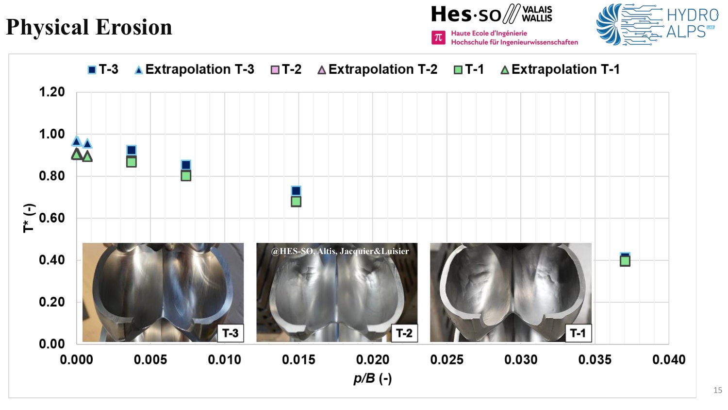
For a healthy runner the dimensionless torque rises toward the target as the particles shrink, and a linear extrapolation to zero particle size lands close to it. That means a fast, coarse run can be used to estimate what a very fine one would give.
Artificial erosion follows the known trends
Flat, rounded and cut-out erosion reproduce the analytical and published efficiency drops, more closely with finer particles. A rounded erosion collapses onto a laboratory experiment on another turbine at another scale, which hints that the effect may not depend on runner size. The worn splitter tip is the exception: the particles are as large as the eroded layer.
Real erosion: the loss comes early
Three real runners were computed: new, after three years, after five (when the owner refurbished). The torque decrease is predicted accurately, and mid-life is already close to end-of-life: torque drops of 6 % and 6.6 % for the mid-life and end-of-life runners, “we have already lost the main part of efficiency even at stage T2”.
“It could be one flood event that can make this high level of erosion. So after one flood event, we lost 2%. It’s not a progressive phenomenon.”
Jean Decaix 22:19 Watch this moment
In short
- Torque loss is predicted, which lets an owner decide whether to refurbish in February or November.
- Next: partial load, where the drop should be larger, then a runner whose speed responds to load rejection.
- A brick of a digital twin: what does 2 % of efficiency lost to one flood cost over a year?

Simulation of Sand Separation and Wear in the Börger FlowSep
A sand separator for biogas plants, simulated before its second prototype: the model showed where the sand escapes, why more flow is worse, and where the housing wears.
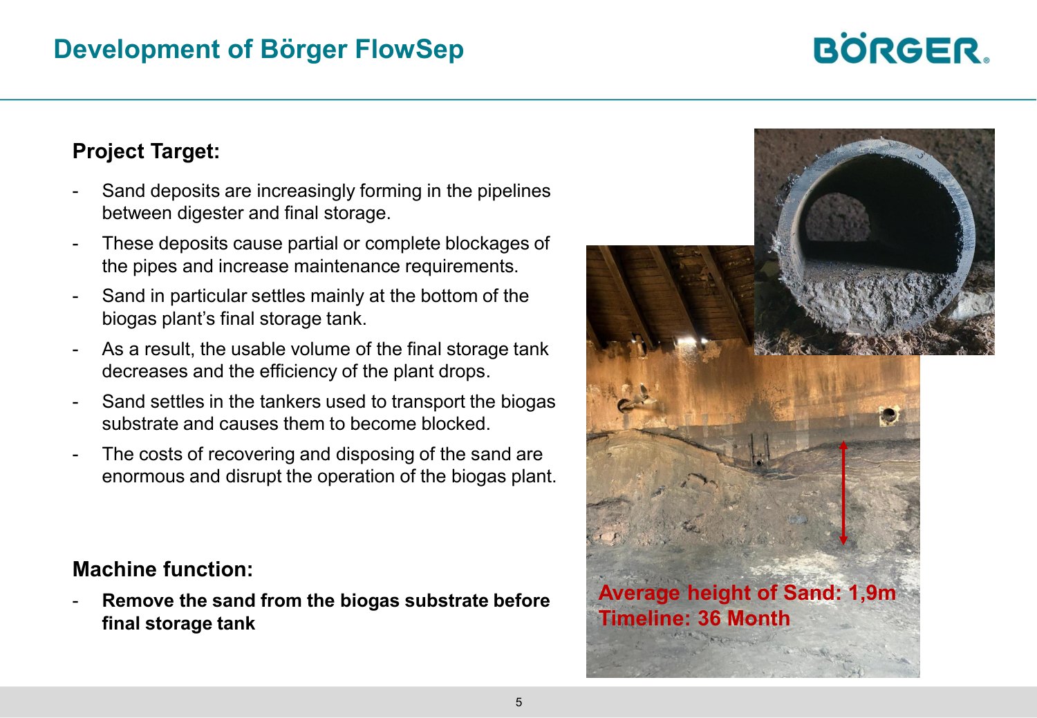
Biogas plants used to be fed with energy crops, a clean medium. Today they run on manure, and with it come sand, stones and soil. In the example shown, 1.9 m of sand settled in 36 months in a 16 m tank: about 1,000 tons. It blocks pipes, defeats the mixers, shrinks the usable volume, blocks the slurry tankers, and is expensive special waste to dig out.
Börger’s BioSelect separator already removes fibres larger than 0.5 mm. The new FlowSep adds centrifugal forces to remove the sand below that size before the final tank. The first mock-up worked immediately; the open questions for the prototype were the geometry, the throughput that still gives an acceptable result, and where the machine wears. EnginSoft built a Particleworks and Granuleworks model, with Börger measuring flows, densities, ash content (burnt at 800 °C) and particle fractions.
Where the sand escapes
About 10 % of the sand leaves through the clean outlet, close to what the tests showed, and only the small particles: large ones are centrifuged outward, as intended. The model shows the path: particles pushed onto the back plate recirculate, and where two opposed fluxes meet a particle that drifts slightly is sucked out with the water. That points straight at a geometry change.
“In a timeline of 36 months, they have had an average of 1.9 meters height of sand. [...] In a container with a diameter of 16 meters, we are talking about 1,000 tons of sand.”
Bernd Valtwies 5:53 Watch this moment
More flow, less separation
Börger’s first idea was to raise the flow rate. At twice the flow the sand not separated grows from about 10 % to about 25 %, with more of the coarse fraction reaching the clean phase. “It’s better to go slower and separate better”, or change the geometry: radius, length, motor size.
“At the beginning, the idea of Börger was: let’s just increase the flow rate, we will be faster, everything will be good. But then, with this simulation, we realized that it’s not possible. It’s better to go slower and separate better.”
Riccardo Sala 25:44 Watch this moment
Where the housing wears
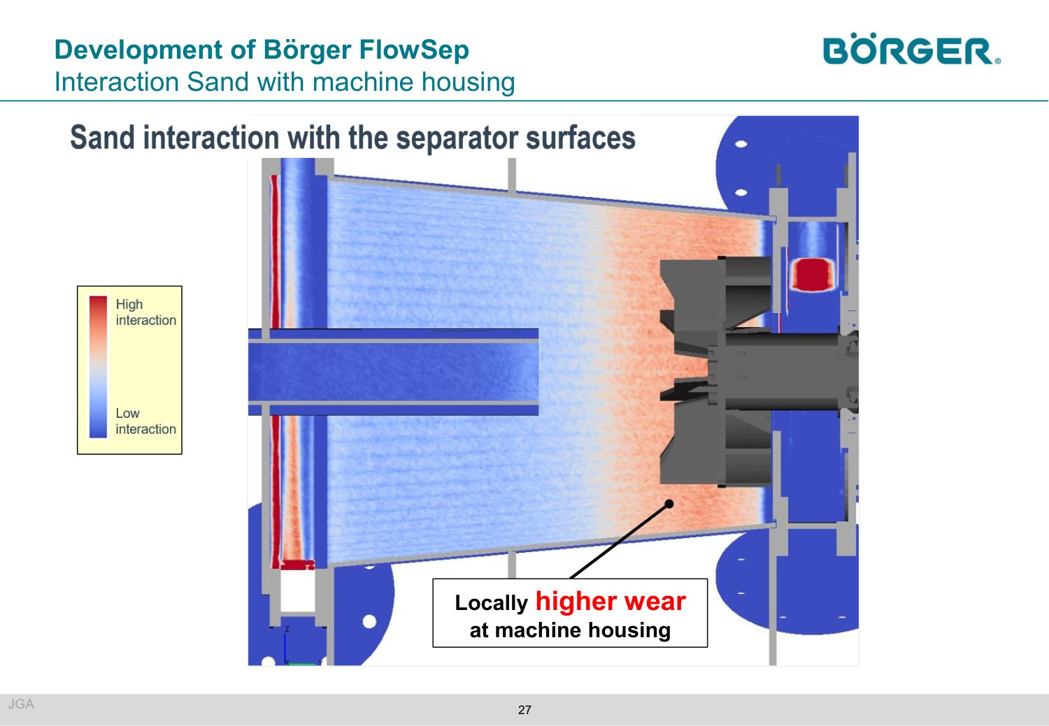
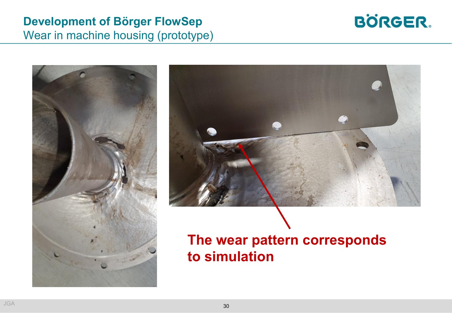
Wall interaction was read from the particle number density within 1 mm of the wall together with velocity. It flags the area near the blades and the back plate, and the prototype, after about half a year of round-the-clock operation, showed strong erosion exactly there. With version 9 the force on the wall is the more direct indicator.
Fewer prototypes
Each prototype costs a lot, and the simulation says early which change makes sense, widening the radius or lengthening the unit, before steel is cut.
In short
- Of the sand that escapes, the small particles are the problem; the geometry can be changed to catch them.
- Higher flow rate: bad separation 10 % → 25 %.
- Simulated wear zones match the prototype: blades and back plate.
Three talks with slides only
These speakers released their slides but not a recording, so there are no quotes here. Each is in the proceedings.
- Prometech Software (Issei Masaie and Iori Saigo) presented the Particleworks 9.0 and Granuleworks 4.0 releases. The new features get their own article.
- IAV (René Kockisch) followed air bubbles in the gear oil of an electric 3-speed commercial-vehicle drivetrain: formation, transport, coalescence and dissolution, measured with the IAV Particle Explorer.
- Univance (Naohiro Fujita) showed gearbox lubrication studies in early design, and early R&D on how airflow changes the oil distribution.
The questions that mattered
What the day showed
Four findings
- Thermal models closed with a steady CHT. Two talks solved oil and metal on separate clocks, in minutes to a day per case, and stated the gap to the bench: about 5–6 °C worst on the pump, up to about 12 % on the roller oil.
- The reading point changes the number. On one sphere the same code returned an HTC of 66 or 169 W/m²K depending on where it was sampled. One air content, 0.65 %, hid bubbles of 132 µm or 68 µm.
- Calibrate on measured bubbles. Optical bubble data took a gearbox aeration model from 0.12 % to 0.45 % air against 0.43 % measured, and from 800 to 186 µm bubbles against 180 µm.
- Simulation also says what not to do. Pelton torque loss and the wear zones of a separator housing were predicted. Doubling the separator flow rate, the obvious fix, raised the sand lost from 10 % to 25 %.
No talk claimed a perfect match. The useful part was the stated gap: about 5–6 °C at worst on the pump, about 12 % on the roller oil, a factor of 2.5 on a sphere depending on where the HTC was read.
Get the Modena proceedings
Slides, recordings and key findings of each released talk. Free, after a short form.
Get the proceedings